Home Blog Page 12

Guide to Contacting Your Member of Congress

0

“`html

Guide to Contacting Your Member of Congress

Contacting your member of Congress remains one of the most measurable forms of constituent input in a system where reelection hinges on district-level sentiment and statewide polling averages. In an environment where approval ratings often swing by double digits between election cycles, direct outreach can shape how lawmakers calibrate their positions ahead of the next map redraw.

Identifying your representatives starts with the official zip-code tools on House.gov and Senate.gov, which pull up not only names and committee assignments but also voting histories that line up with primary and general election data. These resources reveal the 100 senators and 435 House members tied to specific geographies, letting voters cross-reference recent roll calls against demographic breakdowns in their own districts. When you model this electorally, patterns from past cycles show that members in competitive seats pay closer attention to localized feedback than those in safely partisan strongholds.

House members average roughly 760,000 constituents and tend to prioritize infrastructure or district-specific projects, while senators track broader statewide trends that often mirror national polling on White House priorities. The polling data here paints a complicated picture: outreach focused on one chamber can register differently in Senate battlegrounds versus House districts with shifting suburban or rural voter blocs.

Understanding the structural differences between how House and Senate offices operate is crucial for effective communication. House members face elections every two years, making them acutely sensitive to constituent feedback throughout their entire term. Senate offices, operating on six-year cycles, often build more elaborate systems for processing constituent mail because they handle larger volumes over longer periods. A House office might dedicate one or two staffers to constituent services, whereas a senator’s state office infrastructure typically includes multiple regional outreach coordinators. This structural reality means timing your contact with Senate offices around legislative deadlines often yields faster responses, while House members may show more immediate reactivity to sustained grassroots pressure.

Multiple contact channels exist, yet historical patterns indicate phone calls generate the strongest staff logging and internal summaries. Email forms and postal letters create permanent records that offices reference during markup periods, while social media tags can amplify visibility in the weeks before Election Day. Demographic splits matter in how these messages land—urban districts often see faster digital response rates, whereas rural areas still favor traditional mail that tracks with older voter cohorts.

Each contact method carries distinct advantages and limitations worth understanding. Phone calls to a member’s district office typically connect you with constituent services representatives who immediately log your position on specific issues. These calls generate internal tally sheets that staffers review during morning briefings, particularly on legislation under active consideration. A single call might represent “one constituent contact” but can influence how an office weighs constituent sentiment on close votes. Email forms on official House and Senate websites route directly to digital records systems, creating searchable databases that staff reference during briefing preparation. These records prove especially valuable during markup sessions or floor votes, where legislative aides can quickly pull data on constituent input. Postal mail, while slower, carries psychological weight—offices recognize that citizens investing time and postage represent more committed constituent engagement than a quick online form.

Social media outreach works differently across platforms and member offices. Tagging your representative on Twitter or posting on their official Facebook page creates public-facing pressure, particularly effective during news cycles or election-adjacent periods. However, social media contact rarely enters the formal constituent contact logs that staffers review for legislative decision-making. Instead, viral social media activity signals to members that an issue has gained broader public attention, potentially influencing their communication strategy and media positioning rather than direct legislative calculations.

Best practices center on specificity and timing. Messages that cite exact bill numbers or local impact data outperform vague statements, consistent with studies showing higher response rates when constituent input includes verifiable details. Combining personal stories with nonpartisan statistics strengthens the case, particularly when those arguments align with historical voting records that candidates later defend on the campaign trail. For example, rather than writing “I support infrastructure investment,” a more effective message might read: “H.R. [number] would fund bridge repairs on Route 9, which my morning commute depends on. According to the Department of Transportation, this bridge was last inspected in 2019 and rated at structural concern level.”

The timing of your outreach matters significantly more than many constituents realize. Members of Congress face predictable legislative calendars with identifiable pressure points. Contacting your representative during the week they’re home in district often reaches actual staff members with more availability to process detailed constituent feedback. By contrast, messages arriving during intense Washington legislative weeks may be processed more quickly but less thoroughly. Committee markup schedules, which are published weeks in advance, represent ideal windows for contacting members serving on relevant committees. A constituent reaching out the week before a markup on healthcare legislation has better odds of influencing that member’s position than someone contacting two weeks after the vote occurs.

The political calculus of representation also varies by member circumstances. A representative in a safe district may weight constituent calls differently than one in a competitive race. Similarly, a senator facing reelection next cycle often operates under different constituent service pressures than one six years from the next campaign. Understanding these dynamics helps explain why some offices respond quickly to certain issues while remaining unresponsive on others—it typically reflects the member’s electoral math rather than administrative capacity.

Following up with thank-you notes or attending town halls builds the kind of ongoing relationship that can influence how a member positions themselves during tight election cycles. Town hall attendance, particularly when combined with documented questions or comments, signals deeper engagement than a single phone call. Members’ staff track who attends multiple events, and regular attendees often receive priority consideration when constituent services issues arise. This relationship-building approach proves especially effective for constituents dealing with complex federal issues like Social Security benefits, immigration cases, or federal contract disputes—problems that benefit from a congressional office’s specialized knowledge and connections within federal agencies.

Across 535 total voting members, offices handling thousands of weekly contacts on high-profile issues demonstrate that consistent, respectful engagement still registers in internal tallies used for reelection planning. The cumulative effect of constituent contact—whether through calls, letters, or in-person engagement—creates the constituent sentiment baseline that influences how members calculate their positions on contentious votes. While individual contacts rarely change votes in isolation, patterns of constituent contact across a district or state absolutely factor into how members and their teams assess electoral viability and positioning for future campaigns.
Sources

“`

How the US Electoral College Actually Works

0
How the US Electoral College Actually Works

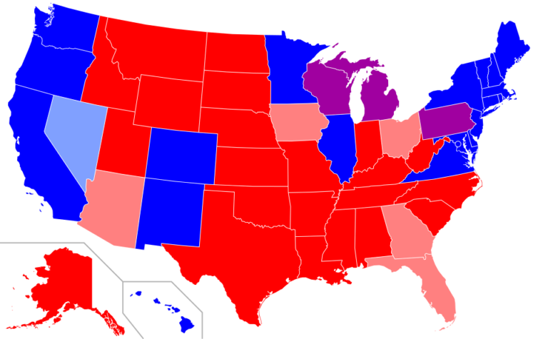
As a Latina journalist covering Washington accountability, I’ve seen how the Electoral College isn’t just some dusty constitutional artifact—it’s a system that quietly steers campaign cash and lobbying firepower toward a narrow slice of battleground states. The US Electoral College serves as the unique constitutional mechanism that ultimately decides who becomes president of the United States, often sparking debate during every presidential election cycle. Unlike a direct popular vote, this system blends state-based representation with federal requirements, requiring candidates to secure 270 electoral votes out of 538 available. Its design reflects compromises made at the Constitutional Convention, balancing interests between large and small states while avoiding pure democracy or congressional selection of the executive.

The financial disclosures tell a story the press releases don’t: super PACs and dark-money groups pour resources into states that can flip the math, while safe strongholds get ignored.

The framers embedded the Electoral College in Article II, Section 1 of the Constitution to create a buffer between the public and the final selection of the president. They worried that direct elections could lead to uninformed choices or regional factions dominating the outcome. Instead, each state appoints electors equal to its total congressional representation—senators plus representatives—plus three for the District of Columbia under the 23rd Amendment.

During the 1787 Convention, alternatives like selection by Congress or state legislatures were rejected in favor of this hybrid approach. The system aimed to protect smaller states from being overshadowed by population centers such as New York or Virginia. Over time, the 12th Amendment refined procedures after the contentious 1800 election, requiring separate ballots for president and vice president.

Alexander Hamilton defended the Electoral College in Federalist No. 68 as a safeguard against foreign influence and unqualified candidates. The process was meant to ensure thoughtful deliberation by electors chosen for their wisdom, though modern practice has largely turned them into pledged delegates following the popular vote in their states.

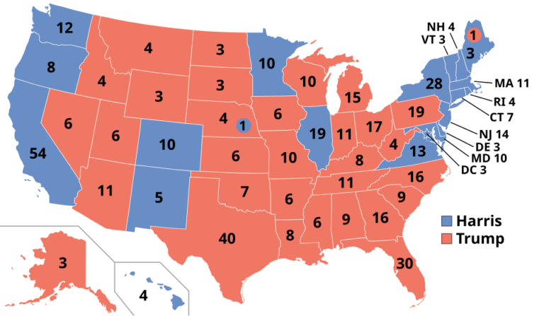
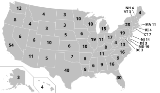
Electoral votes are distributed based on the decennial census, giving California 54 votes while Wyoming receives only three. Most states employ a winner-take-all method, awarding all electors to the candidate who wins the statewide popular vote. This rule amplifies margins in closely contested battlegrounds and explains why candidates focus resources on states like Pennsylvania, Michigan, and Georgia rather than safe strongholds. Campaign finance filings reveal the downstream effect: television ad buys and field operations cluster in those same dozen states, turning electoral math into a multimillion-dollar targeting exercise.

Only Maine and Nebraska allocate electors by congressional district, with the statewide winner claiming the two additional votes tied to senators. This district method has occasionally split a state’s electoral votes, as seen in Nebraska during the 2008 election when Barack Obama secured one vote.

Although rare, faithless electors have cast ballots against their state’s popular vote winner. The Supreme Court upheld state laws binding electors in 2020, reducing the practical impact of such defections. States impose varying penalties, from fines to replacement of wayward electors, to maintain fidelity to voter intent.

Presidential elections occur on the Tuesday after the first Monday in November, followed by the meeting of electors in their state capitals on the first Monday after the second Wednesday in December. Electors submit signed certificates to Congress, where the vice president presides over the joint session on January 6 to count and certify the votes. A candidate needs a majority of 270 to win outright.

If no candidate reaches 270 electoral votes, the 12th Amendment directs the House of Representatives to choose the president from the top three electoral vote recipients, with each state delegation casting one vote. This has happened twice in U.S. history, in 1800 and 1824, highlighting the system’s potential for political maneuvering.

Proposals for a national popular vote compact have gained traction among some states, aiming to bypass the Electoral College without a constitutional amendment. Critics argue the current system discourages turnout in non-competitive states, while defenders emphasize its role in preserving federalism and preventing urban dominance in national outcomes. Lobbying disclosures show that groups pushing reform or defending the status quo often draw funding from the same donor networks that game the existing map.

The total number of electoral votes stands at 538, requiring 270 for victory in every presidential election since the 23rd Amendment. Only three presidents have won without the national popular vote: Rutherford B. Hayes in 1876, Benjamin Harrison in 1888, and George W. Bush in 2000. California holds the largest share with 54 electoral votes, while seven states and the District of Columbia have the minimum of three. Faithless electors have appeared in 10 elections but never altered the final outcome. The winner-take-all system is used by 48 states, concentrating campaign activity in roughly a dozen battleground states. Electors must be at least 18 years old and cannot hold federal office under the Constitution.

The US Electoral College remains a distinctive feature of American democracy that continues to shape presidential campaigns, policy priorities, and national discourse. While it has endured for more than two centuries with only minor adjustments, discussions about its fairness and effectiveness persist. Understanding its mechanics—from state allocation to congressional certification—provides essential context for analyzing election results and potential future reforms. As the nation approaches each presidential election, the system’s influence on strategy and outcomes underscores its lasting constitutional significance.


Sources

How the US Electoral College Actually Works

0

“`html

How the US Electoral College Actually Works

When you model this electorally, the path to 270 votes forces campaigns to prioritize a narrow band of states whose demographic mixes—suburban independents, working-class voters in manufacturing regions, and growing Hispanic populations—can shift outcomes based on turnout models that pollsters refine with likely-voter screens and weighting by education and race. The system itself emerged from Article II compromises that blended population-based House seats with equal Senate representation, yielding 538 total electors today after the 23rd Amendment added three for the District of Columbia.

The framers rejected pure congressional selection or direct popular vote partly to insulate against factionalism, a concern that echoes in modern polling where national popular vote margins often diverge from state-level results. Historical patterns show this tension clearly: the 1800 and 1824 contingent elections in the House, plus the three instances since Reconstruction where candidates prevailed without the national popular vote—Hayes in 1876, Harrison in 1888, and Bush in 2000—highlight how the map rewards efficient geographic distribution over raw totals. The 12th Amendment later required separate ballots for president and vice president, tightening procedures after those early fractures.

Understanding the foundational math behind electoral apportionment helps clarify why certain states dominate campaign calendars. Each state receives a number of electors equal to its total representation in Congress: the number of House members (based on population via the decennial census) plus two senators. This formula means California, with 52 House members and 2 senators, controls 54 electoral votes—roughly 10 percent of the votes needed to win. In contrast, Wyoming, Vermont, and Alaska each have just one House member, giving them the constitutional minimum of three electoral votes. This distribution reflects the founding compromise between large and small states, but it also means that per-capita electoral influence varies dramatically. Wyoming residents exercise roughly 3.6 times the per-capita voting power of Californians when measured by electoral votes per capita, a mathematical reality that shapes both campaign strategy and debates about representational fairness.

Alexander Hamilton’s Federalist No. 68 framing positioned electors as a deliberative check, yet contemporary practice binds them tightly to statewide results in nearly every jurisdiction. Allocation follows the decennial census, so California’s 54 votes contrast sharply with Wyoming’s three, concentrating strategy in battlegrounds where polling methodologies—often blending live calls, online panels, and demographic oversamples—reveal tight margins among white non-college voters and Black turnout cohorts that can decide entire regions.

Most states apply winner-take-all rules, which magnifies small popular-vote edges and explains why resources cluster in Pennsylvania, Michigan, and Georgia rather than safe strongholds. The polling data here paints a complicated picture: repeated surveys across cycles demonstrate how even modest shifts in rural versus metro turnout can flip a state’s entire slate, a dynamic absent in the two states that split electors by congressional district. Maine and Nebraska have occasionally produced divided results, as when Obama captured one Nebraska vote in 2008, underscoring how district-level demographic data can fragment the map.

The winner-take-all system creates a cascading effect that fundamentally shapes campaign priorities. When a candidate wins a state by even a single percentage point, they capture all of that state’s electors. This mechanic means that candidates can theoretically lose the national popular vote by millions while winning the presidency—a scenario that has occurred five times in American history, most recently in 2000 and 2016. Conversely, winning a state by 20 percentage points yields no additional electoral reward compared to winning by one point. This creates powerful incentives for campaigns to ignore demographically safe states entirely. A Democrat commanding 70 percent support in New York receives the same 29 electoral votes as a Democrat winning with 51 percent, while that same candidate struggling in a 48-52 percent race in Arizona faces an all-or-nothing outcome. The result is that roughly three-fourths of the country receives minimal campaign attention in any given election cycle.

Campaign managers rely heavily on historical turnout data and demographic forecasting to identify persuadable voters in swing states. Political scientists have documented that these voters—often called “persuadables” or “moveable middle”—tend to cluster in suburban and exurban areas experiencing demographic transition, particularly collar counties around major metropolitan areas in battleground states. In Pennsylvania, counties like Chester, Bucks, and Delaware have shifted from reliably Republican to highly competitive in recent cycles. In Michigan, counties surrounding Detroit have seen similar trending. Pollsters weight surveys to reflect expected turnout among these populations, though prediction errors in turnout models have repeatedly surprised analysts, as demonstrated in 2016 when models underestimated rural turnout in Midwest states.

The December meeting of electors themselves represents an often-overlooked formal step in the process. While Americans vote on Election Day in November, the actual transfer of power depends on electors meeting in their respective state capitals in December—typically the first Tuesday after the second Wednesday in December—to cast their official ballots. These meetings are ceremonial in most cases, but they provide a final constitutional checkpoint. The electors then send their tallies to Congress, which convenes on January 6 to officially count the votes in a joint session, with the vice president presiding in their role as president of the Senate.

Faithless electors remain statistically rare across ten elections and have never changed a final tally; the Supreme Court’s 2020 ruling upholding state binding laws further reduced their leverage. Certification flows from November’s Tuesday election through December’s state capital meetings and the January 6 joint session, with the 270-vote threshold intact since the current apportionment.

The historical contingent election process, by which the House selects a president when no candidate reaches 270 electors, has not been invoked since 1824, but it remains part of the constitutional design. Should no candidate reach that majority, the House chooses from the top three with each state delegation holding one vote—an arrangement that would require negotiation among state delegations and could theoretically produce outcomes divorced from popular preferences. This scenario becomes more plausible if third-party candidates gain electoral votes in a fragmented election, a concern that influenced strategic voting patterns in elections featuring prominent independent or third-party contenders.

Proposals for a national popular vote compact among states attempt to circumvent constitutional change, yet defenders note the system’s role in preserving federal balance, a point reinforced by historical election data showing how non-competitive states see depressed turnout in demographic subgroups that pollsters track through longitudinal panels. The National Popular Vote Interstate Compact has been adopted by states controlling 209 of the 270 needed electoral votes as of 2024, representing a strategy to ensure that presidents are elected by national popular vote margins without requiring a constitutional amendment.

Key structural facts remain consistent: 538 electors total, minimum three votes for seven states plus the District of Columbia, winner-take-all in 48 states, electors barred from holding federal office, and campaign focus narrowed to roughly a dozen battlegrounds. These mechanics continue to shape both polling interpretation and strategic resource allocation across successive cycles. For voters and observers seeking to understand presidential elections, recognizing these structural features—how census reapportionment shifts electoral power between regions, why certain states consistently attract campaign resources while others are ignored, and how razor-thin margins in a handful of states can determine national outcomes—provides essential context for analyzing both electoral strategy and the broader debate about representational fairness in American democracy.


Sources

“`

Dark Money Networks and Their Sway Over Congressional Campaigns

“`html

Dark Money Networks and Their Sway Over Congressional Campaigns

Campaign finance dynamics in recent cycles have highlighted how undisclosed contributions move through nonprofit channels and hybrid vehicles, shaping outcomes in competitive congressional districts without direct voter visibility into donor sources. Independent trackers document this spending as a recurring element in both primaries and generals, with notable concentration in battlegrounds where control of the House or Senate often hinges on narrow margins.

The legal framework allowing limited disclosure stems from longstanding tax provisions and court precedents that balanced advocacy rights against transparency mandates. This setup lets certain organizations engage politically while shielding contributor details, a pattern that has held across multiple election cycles regardless of which party holds power. The Supreme Court’s 2010 Citizens United decision marked a watershed moment, removing restrictions on independent political spending by corporations and unions, which accelerated the growth of organizations designed to exploit disclosure loopholes while maintaining tax-exempt status.

### 501(c)(4) Organizations and Layered Funding

Social welfare nonprofits can conduct advocacy that stops short of their main activity, filing minimal donor data with the IRS. Analyses from recent cycles show these groups directing substantial resources toward issue ads and turnout efforts in targeted districts. When layered with Super PACs that must report some contributors but can accept upstream grants from opaque sources, the result is multiple degrees of separation that complicate tracing ultimate influence.

The mechanics of this layering operate through shell structures where one 501(c)(4) transfers funds to another, or routes money through limited liability corporations (LLCs) that have no formal disclosure requirements whatsoever. A donor writing a check to an LLC can remain completely anonymous, with that money then funneled to a 501(c)(4), which in turn funds a Super PAC’s media buys. By the time the advertisement appears on television, the original source has vanished behind three or four organizational entities. IRS regulations permit 501(c)(4)s to spend unlimited funds on political activity as long as it doesn’t constitute their primary purpose—a threshold that remains largely unpoliced due to resource constraints at the agency.

Research from campaign finance watchdog groups indicates that a single dark money organization can spend tens of millions in a cycle while disclosing fewer than a dozen major donors to any public database. This contrasts sharply with candidate committees, where every contribution above $200 must be itemized with the donor’s name, address, and employer, creating a public record accessible within days.

### Spending Patterns on the Electoral Map

Aggregated data place hundreds of millions in annual undisclosed expenditures, with sharp spikes in the closing weeks before Election Day. These flows cluster in swing states and House battlegrounds involving vulnerable incumbents or open seats, following historical precedents where outside money amplified in low-turnout environments. The polling data here paints a complicated picture: while aggregate national surveys often show limited direct voter awareness of funding sources, granular demographic breakdowns in key suburban and rural districts reveal shifts in turnout models that correlate with late media saturation.

When you model this electorally, the per-voter impact appears comparable across chambers despite differing totals—House races in compact districts can match the intensity of larger Senate statewide efforts. A House district with 400,000 voters receiving $5 million in dark money ads experiences a different saturation level than a Senate race in a state with 5 million voters receiving $20 million. The concentration effect matters; smaller, more homogenous districts can tip from modest spending levels, while Senate races require larger absolute figures to achieve equivalent messaging penetration.

Historical patterns from prior midterms indicate such spending frequently targets moderate candidates in both parties during primaries, accelerating turnover in competitive zones. This dynamic has measurable consequences: districts that experienced sudden spending surges saw higher rates of incumbent defeat or voluntary retirement compared to similarly competitive districts without such intervention. The timing of these expenditures—typically compressed into the final 60 days—minimizes opportunity for counter-messaging from candidate committees operating on smaller budgets.

### Recruitment Incentives and Policy Alignment

Access to these networks can lower barriers for aligned candidates while raising them for others building from traditional small-donor bases. A candidate with strong backing from dark money networks can launch a credible campaign with minimal fundraising infrastructure of their own, since outside groups handle much of the media spending. This advantage proves especially pronounced in primary elections, where name recognition is lower and persuasion is more fluid. Conversely, candidates without such backing must invest heavily in early fundraising or risk being outspent once dark money groups mobilize.

Post-election, legislative focus in committees handling regulation, taxation, and energy has often tracked themes advanced by high-volume issue groups, consistent with trends observed since the expansion of independent expenditures. Members who benefited from substantial dark money support during their campaigns frequently serve on committees where policy decisions directly affect their funders’ interests. While correlation does not prove causation, voting patterns on regulatory matters show notable alignment between recipients of dark money support and the policy priorities of the groups funding them, particularly in industries like energy, telecommunications, and pharmaceuticals.

Bipartisan examples include accelerated retirements or primary challenges in districts experiencing sudden spending surges. When a member votes against the preferences of major dark money funders in their district, subsequent cycles often see challenger recruitment and funding suddenly materialize from previously inactive networks. This pattern suggests sophisticated coordination between external funding sources and recruitment strategies, though proving explicit coordination remains legally complex given coordination restrictions between outside groups and candidates.

### The Role of Trade Associations and Membership Organizations

Beyond traditional nonprofits, trade associations and membership organizations function as additional dark money conduits. Unlike 501(c)(4)s, trade associations registered as 501(c)(6) entities have even fewer disclosure requirements. A pharmaceutical trade group can spend millions on election-related activities while disclosing virtually nothing about funding sources or recipient candidates. This vehicle proves particularly attractive for business-oriented dark money because it maintains the facade of industry representation while functioning as a political spending arm.

Membership dues flowing into these organizations are not itemized anywhere; a company pays its annual dues, and the organization’s leadership decides how much goes to political spending. Voters have no way of knowing whether their healthcare premiums are partially funding political campaigns, or which specific candidates benefit from industry group spending.

### Disclosure Gaps and Enforcement Challenges

Jurisdictional divides between the FEC and IRS create enforcement lags, preserving pathways for multi-entity transfers. The FEC, responsible for enforcing campaign finance law, operates with a budget roughly equivalent to a mid-sized police department covering an activity involving billions of dollars. The IRS, responsible for ensuring 501(c)(4)s comply with the “primary purpose” rule, has minimal staff dedicated to political organization oversight. This structural understaffing means investigations move slowly and violators face delayed consequences, if any.

Proposals for threshold-based donor reporting or transfer restrictions have surfaced repeatedly, yet progress stalls along familiar partisan lines. Transparency advocates propose requiring disclosure of donors above certain thresholds to 501(c)(4)s and other tax-exempt groups, while opponents argue such requirements constitute invasive information collection. Other proposals would require organizations receiving dark money to disclose their sources before spending funds in elections, but this too faces constitutional challenges and partisan opposition from whichever party benefits most from opacity in a given cycle.

Tracking organizations note parallel growth in outside spending relative to candidate committees in both chambers, a shift that echoes earlier realignments in campaign finance without clear partisan monopoly. In some cycles, Democratic-aligned dark money networks outspent Republican counterparts; in others, the reverse occurred. The structural advantage flows to whichever coalition can attract more large donors to undisclosed conduits at any given moment.

### Understanding the Voter Impact

Overall, these patterns underscore a structural evolution in how resources reach the electoral map, with implications for polling accuracy in demographics where turnout proves decisive. Voters in competitive districts often see dramatically different advertising messages than their counterparts in safe districts, creating parallel political realities shaped by invisible funding sources. This fragmentation complicates efforts to build shared understanding of political issues and candidates, as different segments of the electorate receive information funded by different anonymous networks with different agendas.


Sources

Governor Races in Swing States: A Data-Driven Analysis

“`html

Governor Races in Swing States: A Data-Driven Analysis

Competitive gubernatorial contests in battleground states expose more than voter mood swings—they highlight how money flows through state-level power structures, often deciding whose priorities shape taxation, education funding, and regulatory oversight. While analysts pore over approval ratings, unemployment gaps, and suburban trends, campaign finance records reveal the quieter machinery at work: who bankrolls the visibility on infrastructure projects and who gets drowned out.

As a Latina journalist covering Washington accountability, I’ve seen how these state races serve as testing grounds for national donor strategies, with lobbying disclosures frequently showing industry groups pouring resources into executive contests that influence everything from energy policy to border-related spending.

Pennsylvania stands out for its razor-thin margins, where rural conservative pockets clash with growing suburban blocs around Philadelphia and Pittsburgh. Voter-file data shows independent moderates tipping scales under three points, but the financial disclosures tell a story the press releases don’t: manufacturing and energy sector donors have consistently backed incumbents whose records align with favorable tax treatments, creating a feedback loop that correlates with employment metrics in those corridors.

Arizona’s rapid demographic shifts—rising shares of college-educated residents in urban and exurban zones alongside entrenched rural voters—alter traditional alignments. Polling aggregates flag border security and water management as flashpoints, yet lobbying filings from real-estate and agribusiness interests disclose heavy spending aimed at candidates who can steer state budgets away from stricter resource regulations.

Aggregated surveys across cycles confirm that governors polling below 45 percent approval face steeper challenger odds. Demographic splits by education level matter, with turnout models now factoring early and absentee voting patterns. Key blocs include suburban women aged 35-54, working-class independents in manufacturing areas, and Latino participation rates in expanding metros—groups whose mobilization often hinges on which side can sustain ad buys through the final weeks.

Incumbents draw on name recognition and appointment powers, but state unemployment running more than 1.5 points above national averages erodes those edges in regression models. Challengers push cost-of-living and public-safety messages, seeking crossover endorsements to expand reach. Here, the numbers from campaign finance disclosures are stark: established officeholders frequently maintain better than 2-to-1 fundraising advantages, allowing them to frame narratives around projects while opponents struggle for equivalent visibility.

The 2024 and 2026 cycles underscore how gubernatorial contests in swing states increasingly mirror presidential dynamics. Wisconsin, Michigan, and Nevada have emerged as laboratories where both parties test messaging strategies months before statewide federal elections. Early voting infrastructure, voter registration drives, and ground-game operations built for governor’s races often remain in place for subsequent contests, creating structural advantages that ripple across the political calendar. Campaign operatives from both parties treat these races as recruitment pipelines—successful candidates frequently transition to Congress or higher office, while staffers gain experience managing media buys and voter contact at scale.

Economic conditions function as a baseline predictor in gubernatorial races. Research from state political tracking firms shows that when gross state product growth lags national averages by more than two percentage points over a two-year period, incumbent approval ratings typically decline by 4-6 points. This effect proves particularly pronounced in manufacturing-dependent states where factory closures or automation shifts hit hard and visibly. Pennsylvania and Michigan voters in 2024 weighted jobs and wages heavily, with exit polling revealing that kitchen-table issues outweighed cultural messaging among persuadable voters by roughly 2-to-1 margins.

Healthcare policy has become an unexpected flashpoint in several swing-state governor’s races, diverging from traditional assumptions that health issues fade below economic concerns. State Medicaid expansion decisions, prescription drug affordability, and maternal healthcare access generate substantial voter interest, particularly among suburban women and Latino families. Candidates in Arizona and Nevada who emphasized healthcare accessibility logged measurable gains in early polling, suggesting that state-level health bureaucracy—less visible than federal decisions but more directly felt—resonates with midterm voters.

Education funding disputes tied to teacher salaries and school choice initiatives shape contests in ways national media often underreport. Wisconsin and Pennsylvania governor’s races both hinged partly on competing visions for K-12 accountability and charter school expansion. Teachers’ union spending and parent activism around curriculum issues have grown more sophisticated, with micro-targeted digital campaigns reaching specific neighborhoods where school-aged population density runs high. These operations occur largely outside the national news cycle but substantially influence local voting patterns.

Demographic divergence within swing states creates strategic complexity. Arizona’s Phoenix metro area now accounts for roughly 60 percent of state population but maintains distinct political preferences from rural counties that once anchored statewide victories. This geographic spread forces candidates to invest heavily in multiple media markets, each with different cost structures and audience composition. Nevada’s rapid urbanization around Las Vegas and Reno similarly concentrates electoral power in media-expensive zones, raising the financial bar for viable campaigns.

Third-party and independent candidates periodically reshape swing-state gubernatorial dynamics in unexpected ways. While rare winners, strong independent showings can signal voter dissatisfaction with both major-party establishments and occasionally force general-election runoffs or shift coalition strategies. Tracking independent registration trends in Arizona and Nevada reveals pockets where unaffiliated voters now comprise 25-30 percent of active electorate, compared to 15-20 percent a decade ago.

Turnout models have grown increasingly granular, incorporating not just historical participation but also micro-level demographic and behavioral predictors. Data scientists working for state-level campaigns now factor in variables like previous primary participation, donation history, and social-media engagement alongside traditional voter-file metrics. These sophisticated models inform where each campaign allocates field organizers and determines which voter segments receive high-frequency contact. The camps with superior modeling infrastructure—typically those with stronger fundraising—can identify persuadable voters more efficiently, multiplying their advantage in close contests.

These outcomes carry weight beyond state lines. Unified executive-legislative control speeds tax-code changes and education standards, while national party committees watch for signals on future recruitment. Lobbying records from prior cycles show how outside spending in these contests often previews larger federal influence operations, underscoring why tracking every dollar remains essential to understanding who truly holds the levers.


Sources

“`

Forecasting the Fight for House Control Through Data-Driven Midterm Analysis

“`html

Forecasting the Fight for House Control Through Data-Driven Midterm Analysis

House midterm elections have long served as a referendum on the party in power, with decades of Federal Election Commission records and Census-adjusted voting data showing the president’s party routinely shedding 20 to 30 seats when national conditions sour. Rather than chasing any single poll or viral moment, the durable signals come from campaign finance filings, incumbent fundraising advantages, and the quiet work of lobbyists shaping district maps long before voters reach the ballot.

The financial disclosures tell a story the press releases don’t: incumbents clear reelection rates above 90 percent not solely through name recognition, but because their war chests—built with help from PACs and undisclosed dark-money groups—dwarf challengers in most cycles. Open seats created by retirements remain the real battlegrounds, and those contests increasingly hinge on who can tap K Street networks or super PAC bundlers before the maps are even finalized.

As a Latina journalist covering Washington accountability, I see the same pattern repeat across Sun Belt and Rust Belt districts where economic transitions meet aggressive redistricting. Longitudinal analyses of post-census boundaries show that partisan gerrymandering, often enabled by undisclosed lobbying expenditures, reduces the number of genuinely competitive seats while demographic shifts still open unexpected windows in suburban and exurban pockets.

Historical precedent provides a sobering baseline for forecasters. The 2010 midterms saw Republicans gain 63 House seats under President Obama, while 2018 delivered Democrats a 41-seat pickup under President Trump. These swings reflect not just partisan mood but also the mathematical reality that the party controlling fewer seats faces easier pickup opportunities. When one party holds 235 seats and the other holds 200, the majority party’s incumbents face steeper defenses across a wider range of districts. The FEC’s historical compilations reveal that seat swings of 15 to 50 seats are far more common than conventional wisdom suggests, driven by a combination of national conditions, candidate quality, and district-specific dynamics.

Turnout patterns in recent midterms illuminate another critical variable. In 2022, contrary to the historical script predicting heavy losses for the sitting president’s party, Democrats outperformed expectations in part because their voter turnout held steadier than anticipated. Exit polling and post-election analyses showed that abortion rights messaging and inflation concerns cut across traditional partisan lines, pulling independent and suburban voters in ways that older models—built on earlier electoral coalitions—failed to capture. This suggests that forecasting models must remain adaptive, incorporating emerging issues and demographic realignment rather than relying on static coefficients from prior cycles.

Modern forecasting models now blend generic ballot aggregates, special-election results, and econometric variables with one critical addition: campaign finance velocity. When approval ratings for the sitting president dip below 45 percent, historical FEC data show larger seat losses for the president’s party. Fundraising gaps in open seats have correctly predicted roughly 70 percent of outcomes in recent cycles, a reminder that money often moves before voters do.

The mechanics of these financial signals warrant closer inspection. Candidates and their allies file regular FEC reports, creating a monthly window into where resources are flowing. A challenger’s sudden surge in small-dollar online fundraising often signals emerging grassroots energy, while shifts in PAC contributions to previously safe districts can indicate that Washington strategists view the political landscape as shifting. Data analysts tracking these filings in real time have developed early-warning systems that sometimes detect competitive threats weeks before major polling organizations recognize them. The 2018 midterms saw several districts that appeared safe on the basis of partisan lean suddenly flooded with independent expenditure money—a pattern that, had forecasters weighted FEC data more heavily, might have sharpened their predictions.

Turnout differentials between presidential and midterm electorates amplify these effects, with lower participation typically benefiting whichever side has already locked in its donor base. Ensemble models therefore produce ranges rather than single-point predictions, reflecting how late-cycle independent expenditures or last-minute lobbying pushes can still shift narrow majorities. The uncertainty bands around these forecasts often span 10 to 20 seats, a reminder that while directional signals are robust, pinpoint accuracy remains elusive.

District-level demographic change adds another layer of complexity that pure national models struggle to capture. The Census Bureau’s redistricting data and American Community Survey findings show continued migration patterns reshaping electoral baselines. Sun Belt growth, particularly in Texas, Florida, and North Carolina, has shifted House seat allocations, while population declines in the upper Midwest have reduced Democratic opportunity there. These shifts play out over years, creating either tailwinds or headwinds for incumbent parties depending on which demographic groups dominate incoming movers. A district that was 55 percent white in 2010 might be 48 percent white by 2030, a change that typically benefits Democrats but introduces volatility if turnout or coalition composition shifts.

Incumbent strength remains the single strongest variable in House forecasting. Reelection rates above 90 percent persist even in wave elections, underscoring that the structural advantages of holding office—name recognition, constituent service, incumbent’s advantage in redistricting—are formidable. Yet that same incumbency advantage makes open seats the true laboratories of midterm outcomes. When an incumbent retires voluntarily, they typically take their personal brand and relationships with donors with them. Successor candidates must rebuild credibility from scratch, a process that takes time and money. Data from the last three midterm cycles shows that open seats won by the incumbent’s party have shifted by an average of 8 percentage points toward the opposition, a slippage attributable to the absence of an entrenched legislator.

Special elections in the years between midterms offer forecasters valuable early signals. A Republican holding a suburban seat by 55 percent in the district’s last general election might win a special election in that district by 51 percent if national conditions have shifted unfavorably—an early warning that the district is slipping. The 2021 and 2022 special elections revealed vulnerability in seats held by both parties, with some districts showing swings of 8 to 12 points from their presidential or most recent general-election performance. Forecasters who weight these interim contests heavily often detect emerging patterns before traditional polling, which typically ramps up only as a general election approaches.

The structural advantages remain clear: sustained unfavorable economic indicators, combined with lopsided campaign finance disclosures, continue to favor the opposition in off-year contests. Yet the increasing unpredictability of modern electorates—driven by geographic sorting, media fragmentation, and rapid demographic change—suggests that no single model or dataset tells the complete story. The most reliable forecasts integrate FEC filings, polling aggregates, special-election results, and demographic baselines into ensemble frameworks that honestly report uncertainty rather than false precision.


Sources

“`

Pivotal Senate Contests Poised to Shape Congressional Balance

“`html

Pivotal Senate Contests Poised to Shape Congressional Balance

As a Latina journalist covering Washington accountability, I’ve watched how the upcoming midterm elections could tilt the Senate balance, with 33 Class 2 seats on the line and analysts zeroing in on states where recent margins have tightened. Census Bureau figures and past election returns point to suburban expansion and rural mobilization as key variables, but the financial disclosures tell a story the press releases don’t: outside spending from PACs and dark-money networks is already flooding these same districts, often outpacing candidate committees by wide margins.

Historical midterm patterns show the opposition party gaining ground, with the president’s party losing more than five Senate seats on average since 1950. Those trends sharpen in statewide races where economic messaging and federal policy dominate airwaves. Vulnerability metrics based on presidential margins place multiple contests within three points of national averages, giving well-funded challengers openings in areas tied to manufacturing and agriculture data.

Turnout drivers add another layer. Suburban counties have moved an average of four points toward one party across the last three cycles per exit polls, while rural precincts hold steady above 65 percent participation, rewarding candidates who hammer trade and energy. Urban cores swing with national sentiment and often decide races by fewer than 50,000 votes—precisely the margins where last-minute independent expenditures from undisclosed donors can tip scales, as FEC filings from recent cycles already preview.

The mechanics of Senate campaigns in the modern era demand unprecedented sophistication in voter targeting and message delivery. Campaign operatives now employ algorithmic models that cross-reference voter registration files, consumer data, and social media behavior to identify persuadable audiences down to the household level. These microtargeting efforts, combined with television and digital ad buys, create a fragmented information landscape where different voter segments see fundamentally different campaign messages. This splintering of the political narrative makes it harder for traditional polling to capture the full picture of voter sentiment, since surveys may miss the cumulative effect of tailored messaging reaching specific demographic groups in isolation.

The role of early voting and mail-in ballots has fundamentally altered campaign strategy in ways that extend beyond the November election day itself. States with robust early voting windows and no-excuse mail voting—particularly Arizona, Nevada, and parts of the Upper Midwest—now see campaigns beginning their intensive voter contact efforts weeks before the election. Election officials in these states report that anywhere from 40 to 60 percent of votes are cast before Election Day, meaning candidates must front-load their resources and messaging to reach voters as they enter the voting window rather than waiting for a last-minute sprint. This shift rewards campaigns with superior ground infrastructure and earlier fundraising, creating an advantage for incumbents and well-established challengers.

In the industrial Midwest, legacy manufacturing and growing service sectors make voters sensitive to inflation and supply-chain numbers. Recent Senate results here landed within two points, demanding precise outreach to independents. Michigan’s contest, anchored by its automotive workforce and tech corridors, saw 2018 and 2020 margins under 30,000 votes in key metros. Candidates will push federal infrastructure and semiconductor dollars, yet lobbying disclosures reveal heavy spending by auto and chip interests shaping those very priorities. Wisconsin’s rural-suburban split is equally stark: dairy and manufacturing counties back protectionist policies, while Madison and Milwaukee suburbs track national education trends. A three-percent swing in just four counties could decide it, and campaign-finance records show outside groups already reserving airtime in those same media markets.

Pennsylvania and Ohio present additional complexity in the Midwest equation. Pennsylvania’s electorate has aged notably over the past decade, with voters over 65 now representing a higher-than-national-average share of the electorate. This demographic shift compounds concern about healthcare costs and Social Security adequacy, issues that tend to favor whichever party can credibly claim to defend these programs. Meanwhile, Ohio has experienced significant working-class realignment, with union households—traditionally Democratic strongholds—showing increased volatility in their voting patterns across recent cycles. The state’s reliance on manufacturing employment continues to make trade policy a paramount concern among persuadable voters.

Southern battlegrounds reflect rapid population growth and an influx of college-educated migrants reshaping traditional maps. Georgia’s electorate has added more than 800,000 voters since the last cycle, concentrated in Atlanta suburbs where newcomers skew younger and more diverse. Census migration stats confirm these shifts, and past results show high-propensity suburban turnout can neutralize rural strength. North Carolina blends the Research Triangle with coastal and mountain economies; registered independents now exceed 25 percent, underscoring the value of issue messaging. Here, too, PAC filings disclose coordinated spending from both tech and agriculture lobbies targeting the same swing precincts.

The demographic transformation of Southern suburbs deserves deeper examination. Counties like Cobb County (Georgia), Wake County (North Carolina), and Maricopa County (Arizona) have undergone dramatic shifts in their voter composition. Young professionals, many employed in tech and professional services, have relocated to these areas seeking lower costs and quality of life compared to coastal metros. This influx has created a political dynamic where traditional Republican strength in suburban areas faces pressure from an increasingly diverse, college-educated electorate concerned with social issues and environmental policy. These counties are now regularly swing precincts that determine statewide election outcomes, making them the primary target for campaign resources from both parties.

Western races turn on energy production, technology, and water management, often featuring candidates with executive backgrounds. Analytical models that fold in fundraising totals and district-level indicators flag sustained pressure on Arizona and Nevada, where partisan registration gaps remain tight and early voting rates are high. Ground operations focused on ballot curing will matter, but so will the Super PAC and 501(c)(4) money trails that disclosures are only beginning to illuminate.

The issue of voter registration dynamics in Western states cannot be overlooked. Nevada and Arizona have seen dramatic growth in registered independent voters—now comprising 20-25 percent of the electorate in both states—creating an unpredictable element in Senate races. These voters tend to be persuadable but also highly volatile, responding to specific candidate messaging and local conditions rather than national party cues. Campaigns in these states invest heavily in independent voter persuasion, often testing messages around specific policy concerns like water availability, cost of living, and border security to determine which resonates most effectively.

The data on demographics and turnout remain central, yet following the money reveals how outside interests are already positioning themselves for the narrowest contests. Examining contribution patterns from industries with significant regulatory exposure—pharmaceuticals, financial services, energy companies—shows clear concentration of spending in the most competitive races. This alignment between industry interests and tight electoral margins suggests that the outcomes of these Senate contests will likely shape not only the chamber’s partisan balance but also the legislative agenda on issues ranging from environmental regulation to healthcare reform. Voters in these pivotal states should expect to see unprecedented levels of spending and messaging intensity as both parties recognize that control of the Senate hangs in the balance.


Sources

“`

Record PAC Spending Transforms Midterm Election Strategies

“`html

Record PAC Spending Transforms Midterm Election Strategies

In recent midterm cycles, outside spending through PACs has scaled dramatically, reshaping resource allocation in House and Senate contests across the electoral map. Federal Election Commission records track hundreds of millions funneled into competitive districts and states, frequently surpassing direct candidate outlays. This pattern invites scrutiny of how such flows intersect with voter targeting, particularly when layered against demographic breakdowns in battleground areas.

Historical trends show consistent escalation rather than isolated spikes. Independent expenditures have risen by double-digit margins in key races compared with prior cycles, a shift traceable to regulatory adjustments that expanded contribution limits for certain vehicles. Leadership PACs tied to incumbents have broadened their networks, while hybrid structures now blend direct and independent channels in ways that echo adaptations seen in 2018 and 2022. When you model this electorally, the growth appears structural, concentrated in open seats and narrow-margin districts where polling methodology often reveals late swings among suburban and working-class cohorts.

The 2022 midterm elections witnessed unprecedented PAC activity, with outside spending groups collectively pouring more than $2.7 billion into federal races. This represented a substantial increase from the 2018 cycle and underscores a long-term trend accelerated by the Supreme Court’s Citizens United decision in 2010. Super PACs, which can accept unlimited contributions from individuals, corporations, and unions for independent expenditures, have become central players in competitive contests. These organizations operate separately from candidate campaigns but often coordinate messaging and targeting strategies within legal boundaries, creating powerful financial networks that extend candidate reach far beyond traditional fundraising.

Sector contributions further clarify the map. Finance, insurance, and real estate groups lead, followed by health care, energy, and technology. Filings indicate these prioritize Senate races with banking oversight stakes or House panels handling Medicare and drug pricing. Energy interests cluster in states with extractive employment, aligning funds with jurisdictions where historical voting patterns among rural demographics have proven decisive. Such targeting operates more through regulatory alignment than broad ideology, allowing analysts to trace timelines against recipient records in swing districts.

The mechanics of modern PAC spending reveal sophisticated operational structures. Donor networks often span multiple committees—some registered as Super PACs, others as traditional PACs bound by contribution limits, and still others as 501(c)(4) nonprofit organizations that shield donor identities. This layered approach allows major donors to maximize influence while maintaining plausible distance from campaign messaging. Traditional PACs connected to business associations or unions can contribute directly to candidates up to $5,000 per election, while Super PACs face no contribution caps but cannot coordinate directly with campaigns. The distinction matters for campaign strategy, as integrated networks of these entities can dominate advertising and voter contact landscapes in targeted races.

Digital targeting has emerged as a critical dimension of PAC spending allocation. Rather than the broad media buys of previous decades, contemporary PAC strategies emphasize programmatic advertising, social media microsegmentation, and data-driven voter contact. These approaches allow spending groups to identify persuadable voters at granular levels—by precinct, demographic profile, or even individual household characteristics—and deliver tailored messaging. Such precision comes with significant costs, requiring substantial investment in data analytics and media technology. However, the efficiency gains justify the expense for well-funded organizations, permitting concentrated spending in the handful of truly competitive districts that typically determine chamber control.

Empirical correlations link heavy PAC involvement to gains in name recognition and ad volume for backed candidates. In tight races, outside totals frequently eclipse candidate committees, altering messaging control. Challengers with PAC backing post higher success rates in open contests, while incumbents draw on established ties for defensive positioning. The polling data here paints a complicated picture, as early endorsements can suppress primary challenges through resource signals, and coordinated advertising often synchronizes with fluctuations in battleground polling among independent and minority voters.

State-level variations in PAC activity reflect both competitive dynamics and regulatory environments. Senate races consistently attract disproportionate outside spending, as individual states serve as distinct electoral markets with high-stakes implications for chamber control. A single competitive Senate race can draw over $200 million in combined candidate and outside spending, dwarfing most House contests. Governors’ races increasingly mirror this pattern, particularly in purple states where control affects redistricting and electoral administration. Conversely, safe districts—whether solidly Democratic or Republican—receive minimal PAC attention, creating stark geographic disparities in campaign intensity and voter exposure to advertising.

The timing of PAC spending within election cycles reveals strategic decision-making. Early spending often concentrates on primary races, where well-funded groups seek to shape nominee selection by boosting favored candidates or depleting resources for disfavored contenders. As general elections approach, spending patterns shift toward swing districts and competitive statewide races. Late-cycle spending spikes are common, with September and October seeing massive advertising influxes in battleground areas. This temporal concentration means voters in competitive regions experience campaign saturation while those in safe districts see minimal activity, creating information asymmetries that can advantage better-funded candidates.

Disclosure requirements exist, yet real-time gaps remain for hybrid entities, complicating immediate assessment. Aggregators rely on public filings to gauge aggregate effects, though reporting lags limit scrutiny in fast-moving cycles. The FEC requires major spending reports at specific intervals, but the time lag between expenditure and public disclosure can exceed weeks, limiting real-time accountability. Dark money groups, while required to disclose to the IRS, face no obligation to reveal their donors publicly, creating opacity around funding sources for significant campaign spending. Some organizations deliberately structure contributions to minimize transparency—routing funds through multiple entities to obscure ultimate sources. This complexity challenges voters and analysts seeking to understand who funds particular campaigns or messaging efforts.

Political scientists studying PAC impact have identified measurable effects on campaign dynamics. Research indicates that early PAC support for candidates increases their viability perceptions among donors, voters, and political insiders, creating momentum effects that can prove decisive in close primaries. In general elections, PAC spending appears most influential in low-information races—typically House contests where voters lack extensive prior knowledge of candidates. The relationship between spending and electoral outcomes is not purely causal, however, as PAC organizations often fund candidates already positioned to win. Distinguishing between PAC spending driving victory versus funding candidates likely to win regardless remains methodologically challenging.

Proposals for digital enhancements draw from quantitative reviews of spending concentration, underscoring the need for ongoing data platforms to evaluate influence across the map without partisan overlay. Transparency advocates have pushed for real-time disclosure requirements, reduced reporting intervals, and digital platforms that aggregate spending data accessible to voters and researchers. Some proposals target dark money loopholes through enhanced IRS disclosure requirements for 501(c)(4) organizations involved in electoral activity. Others focus on strengthening coordination rules between Super PACs and candidate campaigns. The debate over PAC reform reflects broader disagreements about campaign finance, free speech, and democratic equality, ensuring that spending patterns and their regulation will remain central to American electoral politics.


Sources

“`

The Evolving Landscape of Swing Voters in America’\”s Suburbs

“`html

The Evolving Landscape of Swing Voters in America's Suburbs

Suburban communities remain decisive swing territories on the electoral map, where even small movements in voter coalitions can tip House districts and presidential battlegrounds. Recent census and voter-file data point to steady population inflows, rising shares of college-educated residents, and greater racial diversity across these zip codes, all of which are reshaping the profile of independent and persuadable voters. When you model this electorally, the result is a more fragmented suburban electorate whose priorities on housing costs, schools, and pocketbook issues cut across traditional partisan lines rather than aligning neatly with national messaging.

The polling data here paints a complicated picture of how these shifts play out. American Community Survey figures show suburban counties gaining residents from both urban cores and rural areas, accompanied by higher percentages of Latino, Asian, and Black households alongside an uptick in college-degree holders relative to national averages. Historical patterns from the last three cycles indicate that these demographic changes have broadened the set of issues swing voters weigh, moving beyond simple economic retrospectives toward a mix that also includes education access and local affordability.

Income dynamics add another layer. Median household earnings in many suburban counties now outpace urban centers, yet cost-of-living pressures persist for younger families and empty-nest professionals alike. Voter-registration files reveal that independents in these counties frequently split tickets based on hyper-local concerns, a pattern that echoes earlier cycles when suburban voters decoupled presidential and down-ballot choices. Regression models controlling for age and income continue to find that racial diversity accounts for a statistically significant share of variance in this ticket-splitting behavior.

The suburban swing voter profile has become increasingly heterogeneous in ways that complicate traditional political analysis. Exit polling from recent election cycles reveals that suburban voters now prioritize issues differently based on their stage of life and professional circumstances. Young professionals working in tech or knowledge industries gravitate toward messaging centered on infrastructure investment and climate policy, while parents with school-age children respond more directly to education quality rankings and curriculum transparency. Empty-nesters, by contrast, demonstrate heightened sensitivity to property tax assessments and local government efficiency. This fragmentation means that a single campaign message rarely resonates equally across suburban precincts, forcing campaigns to develop sophisticated micro-targeting strategies that acknowledge these internal divisions.

Demographic movements are occurring on parallel tracks. College-educated women have accelerated into suburban precincts, correlating with heightened attention to reproductive rights and workplace policies, while working-class households headed by non-college-educated men have grown in outer-ring areas, elevating manufacturing and trade concerns. The polling data here paints a complicated picture because these blocs resist easy categorization; multiracial households show elevated support for immigration reforms, remote-work populations flag broadband access, and declining evangelical identification tracks with more moderate stances on social questions. Turnout among newer suburban demographics still lags established residents, but once mobilized these groups respond more readily to targeted economic messaging, a contrast that appears sharper in midterm versus presidential cycles.

Geographic concentration patterns further illuminate suburban political dynamics. Metropolitan areas around Sun Belt cities—Austin, Atlanta, Phoenix, and Charlotte—have experienced the most dramatic demographic transformations, with college-educated in-migration combining with rapid Hispanic population growth to create genuinely competitive terrain. Conversely, older suburban rings around Rust Belt cities face stagnation or population loss, which maintains traditional voting patterns but reduces their overall electoral influence. The most volatile swing districts tend to cluster in mid-tier metros and exurban counties where multiple demographic currents collide: aging populations of union households alongside younger college-educated families, established immigrant communities coexisting with newly arriving international residents. These overlapping demographic layers mean that electoral shifts can occur rapidly as generational turnover accelerates within relatively compact geographic areas.

The role of local governance and municipal services cannot be overstated when analyzing suburban swing voting behavior. Contrary to national campaign narratives, suburban voters frequently base electoral decisions on school district performance, public safety records, infrastructure maintenance, and municipal fiscal health. Campaigns that focus exclusively on federal messaging miss opportunities to connect with swing voters on the issues that dominate their daily civic lives. School board elections and zoning debates often precede presidential cycles in shaping suburban political sentiment, establishing momentum that carries into higher-level contests. Candidates and campaigns that demonstrate detailed knowledge of local issues—property assessment methods, bond measures, teacher compensation frameworks—consistently outperform those relying on generic national talking points.

Educational attainment has emerged as perhaps the single most predictive variable in suburban electoral behavior, surpassing traditional class-based measures in some contexts. College-educated suburban voters, particularly those with advanced degrees, have shifted substantially in recent cycles, with women gravitating toward Democratic candidates at record rates while college-educated men remain more evenly divided. This education-based realignment has redrawn electoral maps in affluent suburban counties that historically voted Republican by comfortable margins. Meanwhile, non-college-educated suburban voters demonstrate greater volatility, remaining persuadable on economic messaging while showing inconsistent voting patterns on cultural questions. The interaction between education, race, and gender creates a complex calculus that defies simplistic categorization.

When you model this electorally, campaigns relying on outdated suburban stereotypes risk misallocating resources across competitive states. Updated voter-file segmentation allows precise outreach on housing and education, issues that cross demographic lines and have produced measurable movement in precinct-level returns from recent cycles. Longitudinal voter-file studies show suburban swing voters holding steady on fiscal moderation while displaying greater volatility on cultural questions, with participation rates among Hispanic and Asian suburban residents narrowing historical gaps with White voters. These trends underscore the need for sustained ground-game investment to capture emerging preferences accurately rather than assuming static coalitions.

Digital infrastructure and broadband access have emerged as unexpected swing issues in exurban and outer-ring suburban areas. Remote-work adoption accelerated during recent years, making reliable high-speed internet a tangible electoral concern for younger families and self-employed professionals relocating to lower-cost suburban zones. Candidates addressing rural broadband expansion and digital equity have found unexpected receptiveness among suburban voters who recognize these services as essential infrastructure comparable to water systems or transportation networks. This technological dimension adds yet another layer of issue complexity that generic national campaigns frequently overlook.

The volatility of suburban swing voters extends to their relationship with political parties themselves. Ticket-splitting remains elevated in suburban precincts relative to national patterns, with voters comfortable supporting candidates from different parties in concurrent races. This suggests that party affiliation carries less weight in suburban decision-making than it does nationally, and that issue-by-issue evaluation remains paramount. Campaigns that attempt to activate strict partisan loyalty often find suburban audiences unreceptive, while those emphasizing candidate-specific credentials and local track records achieve better results. The declining predictive power of party registration in suburban areas has forced campaigns to rethink assumptions about voter persuasion and mobilization.

Looking forward, suburban swing constituencies will likely remain pivotal to electoral outcomes at federal and state levels. The continued diversification of suburban populations, ongoing economic pressures on middle-income households, and the increasing salience of education and quality-of-life issues ensure that these areas will remain competitive and contested. Understanding the genuine complexity of suburban voter preferences—resisting stereotypes, engaging with local concerns, and acknowledging internal diversity—represents essential strategic work for any campaign seeking to build winning coalitions.


Sources

“`

The Methodology Maze: Understanding Election Polling Accuracy Issues

“`html

The Methodology Maze: Understanding Election Polling Accuracy Issues

Election polling remains essential for mapping out battleground dynamics and projecting outcomes across the electoral map, yet the recurring shortfalls between survey projections and final results trace back to stubborn methodological constraints rather than overt partisan tilt. These limitations surface most clearly when we examine how samples are built, who responds, and how adjustments are applied—factors that have repeatedly produced surprises in states like Pennsylvania, Michigan, and Georgia over the past three cycles.

When you model this electorally, incomplete sampling frames immediately complicate forecasts because they struggle to capture the full universe of likely voters amid shifting demographics. Older random-digit-dial approaches once covered broader populations, but the move to blended cell-phone, voter-file, and online panels leaves gaps, especially among younger and lower-propensity voters who cluster unevenly across Sun Belt and Rust Belt districts. Address-based and registration-based frames help close some of those holes, but states with aggressive voter-roll maintenance or strict ID rules still show 10-15 percent shortfalls in coverage, hitting transient and minority communities hardest and injecting uncertainty into district-level estimates.

The shift away from landline-heavy surveying reflects genuine changes in American communication patterns, but it has introduced its own set of blind spots. While roughly 85 percent of U.S. adults now carry cell phones, certain segments—particularly older voters and those in rural areas—remain harder to reach through mobile-only strategies. Pollsters who rely too heavily on online panels drawn from opt-in internet communities may systematically exclude populations with limited broadband access or lower digital engagement, skewing results in ways that aren’t always apparent until after Election Day.

Likely-voter screens add another variable that can swing projected margins in close Senate or House races. Models relying on past turnout history versus self-reported interest produce noticeably different results depending on whether emerging blocs in suburban or exurban areas are included or excluded. Historical patterns from 2016 and 2020 demonstrate how these choices can shift toplines by several points in states where education or age cohorts are narrowly divided. A pollster who assumes 2020 turnout levels will reach different conclusions than one who models 2018 midterm participation, and that single methodological choice can flip the direction of a projected margin in competitive races.

The challenge intensifies when pollsters attempt to account for “shy” voters—respondents who support a candidate but hesitate to admit it in surveys due to social desirability bias or fear of judgment. This phenomenon gained renewed attention after 2016 and again in 2020, though empirical evidence suggests its impact varies considerably by region, candidate, and issue salience. Some analysts argue that modern polling’s transparency about methods and reduced stigma around candid responses have diminished shy-voter effects, while others contend that intensifying polarization has made certain voter segments more reluctant to participate honestly in surveys.

The polling data here paints a complicated picture when nonresponse rates dip below 10 percent, as is now common. Respondents with stronger opinions and higher education levels participate at higher rates, while working families and certain ethnic groups do not, creating skews that persist even after standard demographic weighting. Callback studies and incentive experiments confirm that harder-to-reach voters often diverge on economic and candidate-favorability questions, a pattern that has historically tilted aggregates in Rust Belt contests where turnout among non-college voters proved decisive. Research from organizations tracking polling accuracy has found that when a poll achieves a response rate below 5 percent—increasingly typical in the era of caller ID and survey fatigue—the margin of error effectively widens even when statistical adjustments are applied.

Weighting decisions further influence the map because they must balance variables like age, race, education, and region against Census benchmarks. Over-weighting small cells increases variance, while missing interactions with urban density or income leaves residual bias. Multilevel regression and post-stratification techniques offer finer granularity, yet modest changes in targets can still move state margins by one to three points—enough to alter Electoral College or chamber-control scenarios when several battlegrounds sit within that range. The 2020 Census redistricting cycle added another layer of complexity, as pollsters had to recalibrate their demographic targets based on updated population estimates while contending with significant shifts in regional demographics that weren’t fully captured until years later.

One underappreciated factor in polling methodology involves the treatment of voters who refuse to declare a party affiliation. The growth of independent voters presents real sampling challenges, as partisan-based turnout models struggle to forecast their behavior. Some pollsters weight independents based on historical voting patterns, while others employ separate modeling approaches. This divergence in handling unaffiliated voters has produced notably different results in swing states where independents represent 30 percent or more of the electorate, yet no consensus methodology has emerged across the industry.

Mode effects from the shift to online, text, and interactive voice surveys introduce additional measurement differences, particularly on enthusiasm and third-party support questions. Parallel calibration tests show consistent but modest divergences that matter most in polarized districts where small shifts in reported intensity can affect turnout models. A respondent completing a survey on a smartphone may answer differently than one on a desktop computer, and someone text-responding to a survey prompt may display different patterns than one engaging with a live interviewer. These mode effects are rarely publicized but accumulate across a polling season, potentially creating systematic bias in aggregated forecasts.

Newer addressable panels and passive data collection promise efficiency but risk widening coverage gaps among populations less active on digital platforms, a concern that echoes coverage shortfalls seen in earlier cycles. Some firms now experiment with combining traditional survey data with administrative records—voter history, registration data, and consumer information—to construct more sophisticated models of likely voters. While these approaches can improve accuracy, they also raise questions about privacy and the extent to which behavioral data should inform electoral projections.

The practice of “herding” in published polls—where organizations avoid releasing outlier results that diverge too far from consensus—adds another layer of distortion to the polling ecosystem. Pollsters face reputational pressure to avoid being dramatically wrong compared to peers, creating incentives to stay within established ranges even when their underlying data suggests otherwise. This dynamic can suppress the true range of uncertainty and make aggregate polls appear more confident than circumstances warrant.

Independent evaluations of pollster performance across multiple elections highlight the value of transparency on frames, weighting, and mode adjustments. Aggregators that account for house effects and historical accuracy deliver more stable averages, though even leading organizations can miss when turnout assumptions shift unexpectedly. Organizations like the American Association for Public Opinion Research (AAPOR) publish post-election analyses examining which firms performed well and why, yet these lessons aren’t always incorporated quickly into industry practice. Continued experimentation with real-time diagnostics and response-quality tracking remains the most direct route to tightening uncertainty ranges around state-by-state projections. Ultimately, recognizing polling’s inherent limitations while understanding the specific methodologies behind particular forecasts allows observers to consume electoral data more critically and prepare for the inevitable moments when polls diverge from outcomes.


Sources

“`